modelConstantEvaporation
Extends from AixLib.Fluid.Interfaces.FourPortHeatMassExchanger.
Information
Model of an organic Rankine cycle (ORC) as a bottoming cycle.
The thermodynamic cycle is steady-state while the evaporator and the condenser
can be configured to have first order dynamics.
The fluid stream 1 (using Medium1, port_a1, etc.)
is the evaporator hot fluid, e.g., waste heat,
and the stream 2 is the condenser cold fluid.
The working fluid of the cycle is not based on a typical Modelica medium model.
See the Thermodynamic Properties section of this document for the rational.
Cycle Architecture and Governing Equations
The implemented ORC is modeled based on the simplified cycle shown in the figure below. The cycle has two variants depending on the shape of the saturation lines of the working fluid and ηexp. For any given working fluid, the cycle is fully determined by providing the working fluid evaporating temperature Tw,eva, the working fluid condensing temperature Tw,con, the expander efficiency ηexp, and the pump efficiency ηpum. The superheating temperature difference ΔTsup is minimized, meaning it is zero whenever possible; otherwise it assumes the smallest value not to cause the expander outlet state to fall under the two-phase region, i.e. the "dome". Subcooling after the condenser is not considered. The Thermodynamic Properties section of this document details how these state points are found.
An important assumption is that all heat is dissipated, i.e., the cycle is not controlled by thermal load.
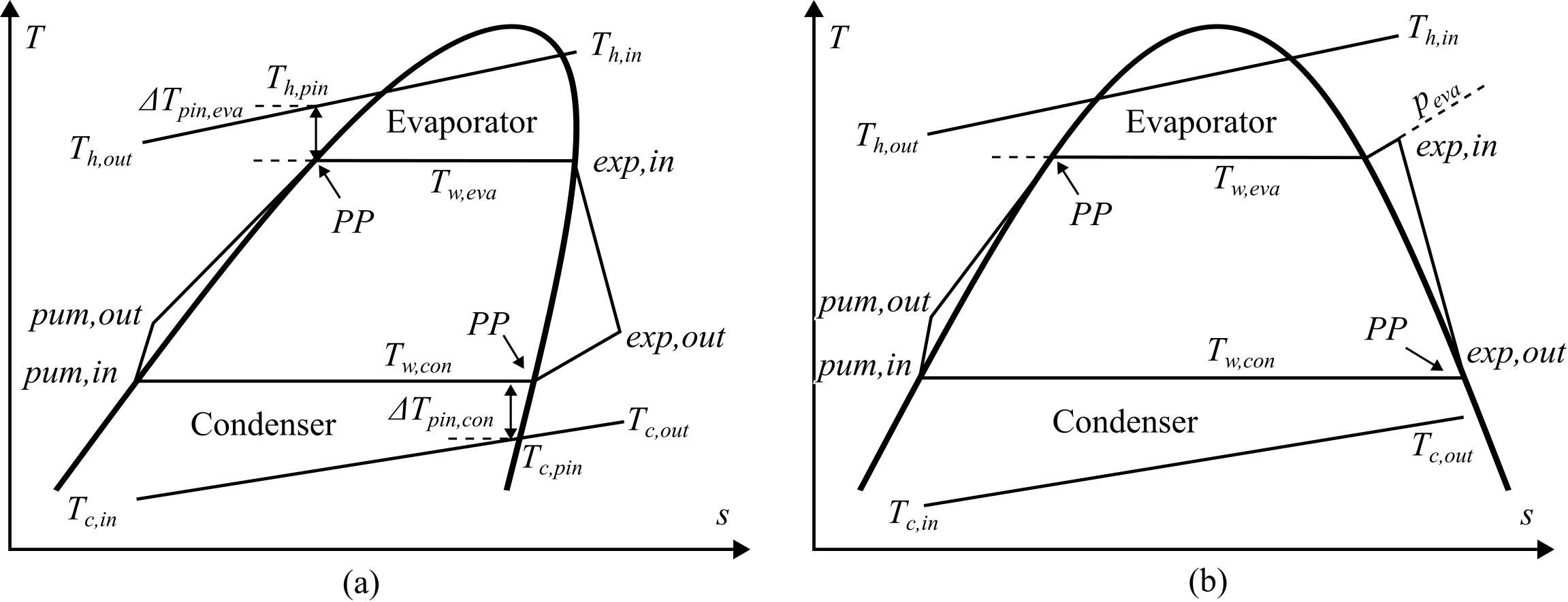
The cycle processes the heat at a fixed Tw,eva provided by the user. The evaporator heat exchange is governed by
Q̇eva = ṁh cp,h (Th,out - Th,in),
Q̇eva = ṁw (hpum,out - hexp,in),
where the subscripts are eva for evaporator, exp for expander, h for hot fluid of the evaporator, i.e. the fluid carrying heat, pum for pump, and w for working fluid.
The cycle accommodates the variable flow rate and temperature of the waste heat stream by changing the working fluid mass flow rate ṁw to maintain a constant pinch point (PP) temperature difference at the evaporator ΔTpin,eva. This difference is found from
(Tpin,eva - Th,out) (hexp,in - hpum,out)
= (Th,in - Th,out) (heva,pin - hpum,out),
ΔTpin,eva = Tpin,eva - Tw,eva.
The condenser side uses the same equations with the evaporator variables replaced by their condenser counterparts where appropriate. Hence,
Q̇con = ṁc cp,c (Tc,out - Tc,in),
Q̇con = ṁw (hpum,in - hexp,out),
(Tc,pin - Tc,in) (hexp,out - hpum,in)
= (Tc,out - Tc,in) (hcon,pin - hpum,in),
ΔTcon,pin = Tw,con - Tc,pin,
where the subscripts are
con for condenser, and
c for cold fluid in the condenser.
The electric power output of the expander is
Pexp = ṁw (hexp,in - hexp,out).
The electric power consumption of the pump is
Ppum = ṁw (hpum,out - hpum,in).
The pump work is
Ppum = ṁw (peva - pcon) / (ρpum,in ηpum).
This takes advantage of the negligible density change of the liquid to avoid a property search in the subcooled liquid region.
In summary, the model has the following information flow:
| User-specified parameters | Inputs | Outputs |
|---|---|---|
|
Tw,eva - Working fluid evaporating temperature, ΔTpin,eva - Evaporator pinch point temperature difference, ΔTpin,con - Condenser pinch point temperature difference, ηexp - Expander efficiency, ηpum - Pump efficiency. |
Th,in - Evaporator hot fluid incoming temperature, ṁh - Evaporator hot fluid flow rate, Tc,in - Condenser cold fluid incoming temperature, ṁc - Condenser cold fluid flow rate. |
ṁw - Working fluid flow rate, Tw,con - Working fluid condensing temperature, Th,out - Evaporator hot fluid outgoing temperature, Tc,out - Condenser cold fluid outgoing temperature, Q̇eva - Evaporator heat flow rate, Q̇con - Condenser heat flow rate, Pexp - Expander power output, Ppum - Pump power consumption. |
Constraints
The ORC system controls ṁw to maintain the prescribed evaporator PP temperature difference set point. Although the model does not implement this as a control loop, an upper limit and a lower limit are imposed on ṁw to reflect the capacity constraints of a sized cycle.
- The working fluid mass flow rate ṁw will not go higher than a prescribed upper limit. Rather, ṁw stays at the user-specified upper limit and ΔTpin,eva increases beyond its set point. This may happen when the incoming hot fluid has a high flow rate or a high incoming temperature, i.e., it carries more energy than the cycle is sized to process.
- When the working fluid mass flow rate ṁw needs to go below a prescribed lower limit, ṁw is set to zero and the cycle is switched off. This may happen when the incoming waste heat fluid has a low flow rate or a low incoming temperature, i.e., it carries too little energy.
How these constraints affect the cycle's behavior reacting to a variable waste heat fluid stream is demonstrated in AixLib.Fluid.CHPs.OrganicRankine.Validation.VariableSource.
Thermodynamic Properties
The thermodynamic properties of the working fluid are not computed by a typical
Modelica medium model, but by interpolating data records in
AixLib.Fluid.CHPs.OrganicRankine.Data.
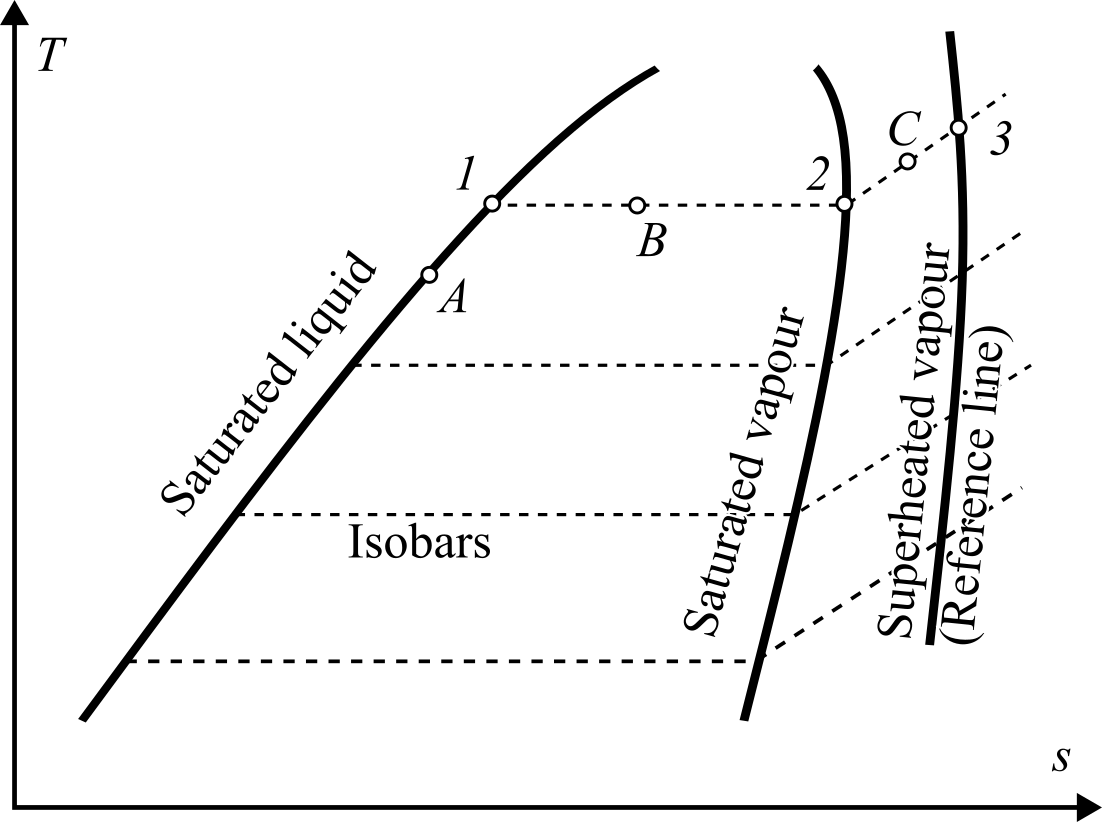
Specific enthalpy and specific entropy values are provided as support points
on the saturated liquid line, the saturated vapor line, and
a superheated vapor line (called the reference line).
The values of these support points were obtained using CoolProp
(https://www.coolprop.org;
Bell et al., 2014) through its Python wrapper and stored as Modelica records.
An example Python file is provided in
AixLib/Resources/Python-Sources/MakeORCFluidRecord.py,
but note that this file is not maintained.
The records included in this library have ten data points for each line.
It is recommended to have at least four points to take full advantage of
the cubit Hermite spline interpolation that is set up in this model.
Thermodynamic state points in the cycle are determined by various schemes of interpolation and extrapolation.
-
On the saturation line, the specific enthalpy, specific
entropy or density, here labeled as yA, are obtained
using cubic Hermite spline interpolation as
yA = s(uA,d)
where s(·,·) is a cubic Hermite spline, uA is the input property, and d are the support points. For the saturation curves, the user can configure the model to use either the saturation pressure or the saturation temperature for uA. For the reference line uA is the pressure. -
If the fluid is wet, the isentropic expander outlet point is in between
the saturation lines. In this case, its enthalpy hB
is obtained from
(hB - h1) / (sB - s1) = (h2 - h1) / (s2 - s1)
where sB is known because it equals the expander inlet entropy, and all other points are on the saturation line and therefore can be found as point A. - C is a point in the superheated vapor region. This is the case for the expander inlet or outlet depending on the shape of the cycle. The isobaric lines are not straight in this section, but they are assumed linear so that the method for B can be applied using the saturated vapor line and the reference line, albeit with less accuracy.
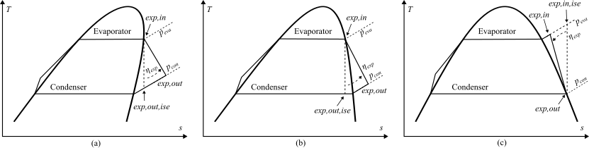
The cycle can be completely defined by providing the following quantities: evaporating temperature Teva or pressure peva, condensing temperature Tcon or pressure pcon, expander efficiency ηexp, and pump efficiency ηpum. Most of the important state points can be found via the interpolation schemes described above. The only exceptions are the expander inlet, expander outlet, and the pump outlet.
-
A dry cycle is a cycle where the expansion starts from
the saturated vapor line and ends in the superheated vapor region.
For either a dry fluid (a) or a wet fluid (b) undergoing such a cycle,
hexp,out - hexp,in = (hexp,out,ise - hexp,in) ηexp
where hexp,out is solved and hexp,in is known. -
A wet cycle is a cycle where the expansion starts from
the superheated vapor region and ends on the saturated vapor line.
In this scenario,
hexp,out - hexp,in = (hexp,out - hexp,inl,ise) ηexp
where hexp,out is known and hexp,in is solved. For this fluid and this ηexp, if the expansion started from the saturated vapor line, the outlet point would end up under the dome.
Implementation
The user can parameterise the evaporating condition by providing either the evaporating temperatureTWorEva or the evaporating pressure
pWorEva. To support this, a default parameter assignment is
provided to both. Otherwise there would be unassigned parameters even though
they are not needed.
References
Bell IH, Wronski J, Quoilin S, Lemort V. Pure and pseudo-pure fluid thermophysical property evaluation and the open-source thermophysical property library CoolProp. Industrial & engineering chemistry research. 2014 Feb 12;53(6):2498-508. https://doi.org/10.1021/ie4033999
Parameters
| Type | Name | Default | Description |
|---|---|---|---|
| AixLib.Fluid.CHPs.OrganicRankine.Data.Generic | pro | ||
| Evaporator | |||
| Modelica.Units.SI.MassFlowRate | mHot_flow_nominal | Nominal mass flow rate of the evaporator fluid | |
| Modelica.Units.SI.PressureDifference | dpHot_nominal | Nominal pressure drop of the hot fluid in evaporator | |
| Modelica.Units.SI.TemperatureDifference | dTPinEva_set | 5 | Set evaporator pinch point temperature difference |
| Boolean | useEvaporatingPressure | false | Set true to specify working fluid evaporating pressure instead of temperature |
| Modelica.Units.SI.ThermodynamicTemperature | TWorEva | max(pro.T)*2/3 + min(pro.T)*1/3 | Evaporating temperature of the working fluid |
| Modelica.Units.SI.Pressure | pWorEva | max(pro.p)*2/3 + min(pro.p)*1/3 | Evaporating pressure of the working fluid |
| Condenser | |||
| Modelica.Units.SI.MassFlowRate | mCol_flow_nominal | Nominal mass flow rate of the condenser fluid | |
| Modelica.Units.SI.PressureDifference | dpCol_nominal | Nominal pressure drop of the cold fluid in condenser | |
| Modelica.Units.SI.TemperatureDifference | dTPinCon | 10 | Condenser pinch point temperature difference |
| Boolean | useLowCondenserPressureWarning | true | If true, issues warning if pCon < 101325 Pa |
| Cycle | |||
| Modelica.Units.SI.MassFlowRate | mWor_flow_max | Upper bound of working fluid flow rate | |
| Modelica.Units.SI.MassFlowRate | mWor_flow_min | Lower bound of working fluid flow rate | |
| Modelica.Units.SI.MassFlowRate | mWor_flow_hysteresis | mWor_flow_min + (mWor_flow_max - mWor_flow_min)*0.1 | Hysteresis for turning off the cycle when flow too low |
| Modelica.Units.SI.Efficiency | etaExp | Expander efficiency | |
| Modelica.Units.SI.Efficiency | etaPum | Pump efficiency | |
Components
| Type | Name | Default | Description |
|---|---|---|---|
| Modelica.Blocks.Interfaces.BooleanInput | ena | Enable cycle; set false to force working fluid flow to zero | |
| Modelica.Blocks.Interfaces.RealOutput | PExp | Expander power generation | |
| Modelica.Blocks.Interfaces.RealOutput | QEva_flow | Evaporator heat flow rate into the cycle | |
| Modelica.Blocks.Interfaces.RealOutput | QCon_flow | Condenser heat flow rate out of the cycle | |
| Modelica.Blocks.Interfaces.BooleanOutput | on_actual | Actual on off status of the cycle | |
| Modelica.Blocks.Interfaces.RealOutput | PPum | Electrical power consumption of the pump | |
| AixLib.Fluid.CHPs.OrganicRankine.BaseClasses.FixedEvaporating | cyc | Thermodynamic computations of the organic Rankine cycle |
Revisions
-
January 29, 2024, by Hongxiang Fu:
First implementation. This is for #3433.