modelCombiTimeTable

Information

This block, derived from the Modelica Standard Library, can read scenarios on a file (see explanation below). The output is a real which may, for example, be connected to a boundary conditions model (prescribing temperature, flow, pressure...).

This block generates an output signal y[:] by linear interpolation in a table. The time points and function values are stored in a matrix table[i,j], where the first column table[:,1] contains the time points and the other columns contain the data to be interpolated.

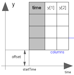
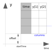
Via parameter columns it can be defined which columns of the table are interpolated. If, e.g., columns={2,4}, it is assumed that 2 output signals are present and that the first output is computed by interpolation of column 2 and the second output is computed by interpolation of column 4 of the table matrix. The table interpolation has the following properties:

• The time points need to be monotonically increasing.
• Discontinuities are allowed, by providing the same time point twice in the table.
• Values outside of the table range, are computed by extrapolation according to the setting of parameter extrapolation:

  extrapolation = 0: hold the first or last value of the table,
                     if outside of the range.
                = 1: extrapolate through the last or first two
                     points of the table.
                = 2: periodically repeat the table data
                     (periodical function).

• Via parameter smoothness it is defined how the data is interpolated:

  smoothness = 0: linear interpolation
             = 1: smooth interpolation with Akima Splines such
                  that der(y) is continuous.

• If the table has only one row, no interpolation is performed and the table values of this row are just returned.
• Via parameters startTime and offset the curve defined by the table can be shifted both in time and in the ordinate value. The time instants stored in the table are therefore relative to startTime. If time < startTime, no interpolation is performed and the offset is used as ordinate value for all outputs.
• The table is implemented in a numerically sound way by generating time events at interval boundaries, in order to not integrate over a discontinuous or not differentiable points.
• For special applications it is sometimes needed to know the minimum and maximum time instant defined in the table as a parameter. For this reason parameters t_min and t_max are provided and can be access from the outside of the table object.

Example:

   table = [0  0
            1  0
            1  1
            2  4
            3  9
            4 16]; extrapolation = 1 (default)
If, e.g., time = 1.0, the output y =  0.0 (before event), 1.0 (after event)
    e.g., time = 1.5, the output y =  2.5,
    e.g., time = 2.0, the output y =  4.0,
    e.g., time = 5.0, the output y = 23.0 (i.e. extrapolation via last 2 points).

The table matrix can be defined in the following ways:

1. Explicitly supplied as parameter matrix "table", and the other parameters have the following values:

   tableName is "NoName" or has only blanks,
   fileName  is "NoName" or has only blanks.

2. Read from a file "fileName" where the matrix is stored as "tableName". Both ASCII and binary file format is possible. (the ASCII format is described below). It is most convenient to generate the binary file from Matlab (Matlab 4 storage format), e.g., by command

   save tables.mat tab1 tab2 tab3 -V4

when the three tables tab1, tab2, tab3 should be used from the model.

3. Statically stored in function "usertab" in file "usertab.c". The matrix is identified by "tableName". Parameter fileName = "NoName" or has only blanks.

Table definition methods (1) and (3) do not allocate dynamic memory, and do not access files, whereas method (2) does. Therefore (1) and (3) are suited for hardware-in-the-loop simulation (e.g. with dSpace hardware). When the constant "NO_FILE" is defined in "usertab.c", all parts of the source code of method (2) are removed by the C-preprocessor, such that no dynamic memory allocation and no access to files takes place.

If tables are read from an ASCII-file, the file need to have the following structure ("-----" is not part of the file content):

-----------------------------------------------------
#1
double tab1(6,2)   # comment line
  0   0
  1   0
  1   1
  2   4
  3   9
  4  16
double tab2(6,2)   # another comment line
  0   0
  2   0
  2   2
  4   8
  6  18
  8  32
-----------------------------------------------------

Note, that the first two characters in the file need to be "#1". Afterwards, the corresponding matrix has to be declared with type, name and actual dimensions. Finally, in successive rows of the file, the elements of the matrix have to be given. Several matrices may be defined one after another.

--------------------------------------------------------------
Licensed by EDF under a 3-clause BSD-license
Copyright © EDF 2009 - 2023
BuildSysPro version 3.6.0
Author : EDF
Initial model : CombiTimeTable, Martin Otter, Copyright © Modelica Association and DLR.
--------------------------------------------------------------

Parameters

Connectors

Contents

Revisions

Release Notes:

• March 31, 2001 by Martin Otter:
  Used CombiTableTime as a basis and added the arguments extrapolation, columns, startTime. This allows periodic function definitions.